Paper - Reinforcement Learning with Deep Energy-Based Policies
This is a brief summary of paper Reinforcement Learning with Deep Energy-Based Policies for my personal interest.
- 0. Introduction
- 1. Motivation
- 2. Soft Definition
- 3. Theorem Analyses
- 4. Algorithm
- 4. Conclusion
- 5. References
0. Introduction
After publishing the paper soft Q learning in Jul 2017, the author proposed the influential algorithm SAC in the next year. While SAC has received tremendous publicity, the discussion, if any, about this precedent work generally falls into the rut of the excellent blog. Therefore I decided to summarize some of thoughts and problems I had during the reading. Though this post is mainly for my personal interest, any advice will be appreciated.
1. Motivation
In reinforcement learning (RL) problem, given an agent and an environment, the objective of the agent is to learn a policy that maximizes the rewards the agent can gain. However, faced with an unknown environment, there is a tradeoff between exploitation and exploration. Before maximum entropy RL, the exploration is generally ensured by external mechanisms, such as \(\varepsilon-\)greedy in DQN and adding exploratory noise to the actions in DDPG. Un like those heuristic and inefficient methods, maximum entropy encourages the agent to conduct exploration by itself based on both reward and entropy. Specifically, in maximum entropy RL, the optimal policy is redefined as
\[\pi^\ast_\text{MaxEnt}=\arg\max_\pi\mathbb{E}_{\pi}\left[r(s_t,a_t)+\mathcal{H}(\pi(\cdot\vert s_t))\right],\tag{1}\]which adds a regularization term to the standard definition. Many paper adds a parameter \(\alpha\) to entropy, which we will ignore in the following discussion as it does not affect the related conclusion. Based on this redefinition, the motivation of this paper can be summarized as follows:
-
Generalize it to continuous cases:
Before this work, entropy maximization was mainly utilized in discrete cases. Theoretical analyses were needed for applying into continuous cases.
-
Take trajectory-wise entropy into consideration:
The term \(\mathcal{H}(\pi(\cdot\vert s_t))\) only considers the entropy of the policy at state \(s_t\). Traditional methods tend to act greedily based on the entropy at the next state. In this work, the author considers the long term entropy reward instead that of the next state.
-
Policy formulation:
Even though we have an objective function given the definition, it still needs a probabilistic definition from which we can make sampling. Instead of using conditional Gaussian distribution like many other works, the author borrows the idea of Boltzmann distribution.
2. Soft Definition
We now discuss the related definition in this paper.
2.1. Objective Function
The optimal policy in this paper is defined as
\[\pi^\ast=\arg\max_\pi\sum_t\mathbb{E}_{(s_t,a_t)\sim\rho_\pi}\left[r(s_t,a_t)+\mathcal{H}(\pi(\cdot\vert s_t))\right],\tag{2}\]which differs from the one defined in \((1)\) as it aims to reach states where they may have high entropy in the future. Specifically, a detailed version is given by
\[\pi^\ast=\arg\max_\pi\sum_t\mathbb{E}_{(s_t,a_t)\sim\rho_\pi}\left[\sum_{l=t}^\infty \gamma^{l-t}\mathbb{E}_{(s_l,a_l)\sim\rho_\pi}\left[r(s_l,a_l)+\mathcal{H}(\pi(\cdot\vert s_l))\right]\bigg\vert s_t,a_t\right],\tag{3}\]where the first expectation \(\sum_t\mathbb{E}_{(s_t,a_t)\sim\rho_\pi}\) is over all the pairs \((s_t, a_t)\) at any time step, and the second expectation \(\sum_{l=t}^\infty \gamma^{l-t}\mathbb{E}_{(s_l,a_l)\sim\rho_\pi}\) is over all the trajectories originating from \((s_t,a_t)\).
In the original paper, the detailed version is actually given by
\[\pi^\ast_\text{MaxEnt}=\arg\max_\pi\sum_t\mathbb{E}_{(s_t,a_t)\sim\rho_\pi}\left[\sum_{l=t}^\infty \gamma^{l-t}\mathbb{E}_{(s_l,a_l)}\left[r(s_t,a_t)+\mathcal{H}(\pi(\cdot\vert s_t))\right]\bigg\vert s_t,a_t\right].\]Problem: The subscripts (shown in red below) in the second expectation does confuse me a lot. Why it is over \(t\) rather than \(l\)?
\[r(s_{\color{red}t},a_{\color{red}t})+\mathcal{H}(\pi(\cdot\vert s_{\color{red}t}))?\]
2.2. Soft Function
The corresponding \(Q\)-function in this paper is defined as
\[Q_\text{soft}^\pi(s_t,a_t)\triangleq r(s_t,a_t)+\sum_{l=t+1}^\infty \gamma^{l-t}\mathbb{E}_{(s_{l},a_{l})\sim\rho_\pi}\left[r(s_{l},a_{l})+\mathcal{H}(\pi(\cdot\vert s_{l}))\right].\tag{4}\]Notice that the entropy at state \(s_t\) is omitted in the definition.
The corresponding value function is given by
\[V_\text{soft}^\pi(s_t)\triangleq \log \int_{\mathcal{A}}\exp\left(Q_\text{soft}^\pi(s_t,a)\right)da,\tag{5}\]which is actually in the form of log sum exponential that approximates maximum.
Given the two definitions, the soft policy is then given by
\[\pi(a_t\vert s_t)=\exp\left(Q^\pi_\text{soft}(s_t,a_t)-V^\pi_\text{soft}(s_t)\right).\tag{6}\]As \(V^\pi_\text{soft}\) only depends on \(Q^\pi_\text{soft}\), the soft policy is actually the Boltzmann distribution based on the value of \(Q^\pi_\text{soft}\). The comparison is shown in Figure 1. It can be found that Boltzmann distribution assigns a reasonable likelihood for all actions (rather than just the optimal one).
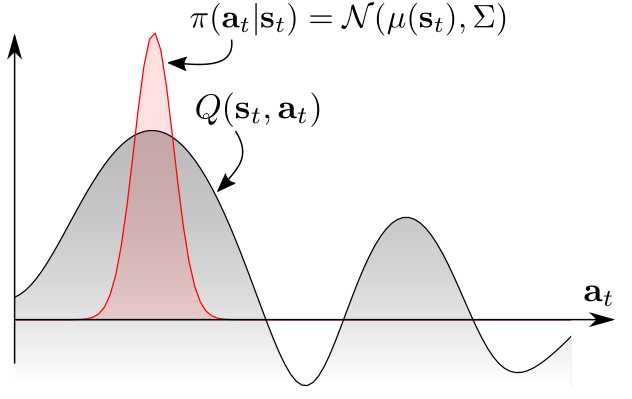
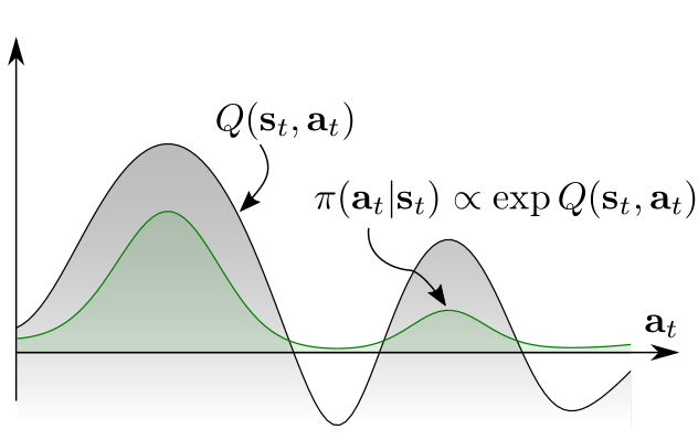
Figure 1. Policies based on the value of Q function. (a) Unimodal policy. (b) Multimodal policy.
With those definitions, we have proposed the solutions to the problems mentioned in the motivation: continuous function for continuous states and actions space; the trajectory-wise optimization defined by the objective function \((3)\); and Boltzmann distribution to represent the optimal policy. To ensure things work, we need theoretical analyses and feasible update rules.
3. Theorem Analyses
We now discuss the related theoretical guarantee. The first theorem shows us the optimality:
Theorem 1: The optimal policy for equation (3) is given by
\[\pi^\ast(a_t\vert s_t)=\exp\left(Q^\ast_\text{soft}(s_t,a_t)-V^\ast_\text{soft}(s_t)\right).\]The proof sketch follows two steps: policy improvement and policy iteration.
3.1. Policy Improvement
We first show that given any policy, we can improve it by ‘softmizing’ it. Specifically,
\[\forall\pi,\text{let }\tilde\pi(\cdot\vert s)\propto\exp\left(Q^\pi_\text{soft}(s,\cdot)\right),\text{then }Q^\pi_\text{soft}(s_t,a_t)\le Q^{\tilde\pi}_\text{soft}(s_t,a_t).\]To show that, we rewrite the second part of \(Q\) function (defined in (4)) as
\[\begin{aligned}&\sum_{l=t+1}^\infty \gamma^{l-t}\mathbb{E}_{(s_{l},a_{l})\sim\rho_\pi}\left[r(s_{l},a_{l})+\mathcal{H}(\pi(\cdot\vert s_{l}))\right]\\=&\mathbb{E}_{(s_{t+1},a_{t+1})\sim\rho_\pi}[[\gamma\mathcal{H}(\pi(\cdot\vert s_{l}))+\gamma r(s_{t+1},a_{t+1})\\&+\sum_{l=t+2}^\infty \gamma^{l-t}\mathbb{E}_{(s_{l},a_{l})\sim\rho_\pi}[r(s_{l},a_{l})+\mathcal{H}(\pi(\cdot\vert s_{l}))]]\\=&\mathbb{E}_{(s_{t+1},a_{t+1})\sim\rho_\pi}[\gamma\mathcal{H}(\pi(\cdot\vert s_{l}))+\gamma (r(s_{t+1},a_{t+1})\\&+ \sum_{l=t+2}^\infty \gamma^{l-t-1}\mathbb{E}_{(s_{l},a_{l})\sim\rho_\pi}[r(s_{l},a_{l})+\mathcal{H}(\pi(\cdot\vert s_{l}))])]\\=&\mathbb{E}_{(s_{t+1},a_{t+1})\sim\rho_\pi}[\gamma\mathcal{H}(\pi(\cdot\vert s_{t+1}))+\gamma Q^\pi_\text{soft}(s_{t+1},a_{t+1})].\end{aligned}\]As the entropy term is independent of \(a_{t+1}\), we then have the following equation
\[Q^\pi_\text{soft}(s_t,a_t)=r(s_t,a_t)+\gamma\mathbb{E}_{s_{t+1}\sim\mathcal{P}}[\mathcal{H}(\pi(\cdot\vert s_{t+1}))+\mathbb{E}_{a_{t+1}\sim\pi}\left[Q^\pi_\text{soft}(s_{t+1},a_{t+1})]\right].\tag{7}\]We then provide an inequality:
\[\mathcal{H}(\pi(\cdot\vert s_{t}))+\mathbb{E}_{a_{t}\sim\pi}\left[Q^\pi_\text{soft}(s_{t},a_{t})\right]\le \mathcal{H}(\tilde\pi(\cdot\vert s_{t}))+\mathbb{E}_{a_{t}\sim\tilde\pi}\left[Q^\pi_\text{soft}(s_{t},a_{t})\right].\tag{8}\]Proof of (8):
We rewrite the left hand side of the inequality
\[\begin{aligned}&\mathcal{H}(\pi(\cdot\vert s_{t}))+\mathbb{E}_{a_{t}\sim\pi}\left[Q^\pi_\text{soft}(s_{t},a_{t})\right]\\=&\mathbb{E}_{a_t\sim \pi}\left[{\color{red}{-\log\pi(a_t\vert s_t)}}+Q^\pi_\text{soft}(s_t,a_t)\right]\\=&\mathbb{E}_{a_t\sim \pi}\left[-\log\pi(a_t\vert s_t){\color{red}{+\log\tilde{\pi}(a_t\vert s_t)-\log\tilde{\pi}(a_t\vert s_t)}}+Q^\pi_\text{soft}(s_t,a_t)\right]\\=&-\mathbb{E}_{a_t\sim \pi}\left[\log\pi(a_t\vert s_t)-\log\tilde{\pi}(a_t\vert s_t)\right]+\mathbb{E}_{a_t\sim \pi}\left[Q^\pi_\text{soft}(s_t,a_t)-\log\tilde{\pi}(a_t\vert s_t)\right]\\=&-D_\text{KL}(\pi\vert\vert\tilde{\pi})+\mathbb{E}_{a_t\sim\pi}\left[Q^\pi_\text{soft}(s_t,a_t)-Q^\pi_\text{soft}(s_t,a_t)+\log\int_\mathcal{A}\exp(Q^\pi_\text{soft}(s_t,a'))da'\right]\\=&-D_\text{KL}(\pi\vert\vert\tilde{\pi})+\log\int_\mathcal{A}\exp(Q^\pi_\text{soft}(s_t,a'))da’.\end{aligned}\]For the right hand side of the inequality, we have
\[\begin{aligned}&\mathcal{H}(\tilde\pi(\cdot\vert s_{t}))+\mathbb{E}_{a_{t}\sim\tilde\pi}\left[Q^\pi_\text{soft}(s_{t},a_{t})\right]\\=&\mathbb{E}_{a_t\sim \tilde\pi}\left[{\color{red}{-\log\tilde\pi(a_t\vert s_t)}}+Q^\pi_\text{soft}(s_t,a_t)\right]\\=&\mathbb{E}_{a_t\sim \tilde\pi}\left[-\log\frac{\exp\left(Q^\pi_\text{soft}(s_t,a_t)\right)}{\int_\mathcal{A}\exp\left(Q^\pi_\text{soft}(s_t,a')\right)da'}+Q^\pi_\text{soft}(s_t,a_t)\right]\\=&\mathbb{E}_{a_t\sim \tilde\pi}\left[-Q^\pi_\text{soft}(s_t,a_t)+\log\int_\mathcal{A}\exp\left(Q^\pi_\text{soft}(s_t,a')\right)da'+Q^\pi_\text{soft}(s_t,a_t)\right]\\=&\log\int_\mathcal{A}\exp\left(Q^\pi_\text{soft}(s_t,a')\right)da’.\end{aligned}\]Since \(D_\text{KL}\ge 0\), we have
\(\mathcal{H}(\pi(\cdot\vert s_{t}))+\mathbb{E}_{a_{t}\sim\pi}\left[Q^\pi_\text{soft}(s_{t},a_{t})\right]\le \mathcal{H}(\tilde\pi(\cdot\vert s_{t}))+\mathbb{E}_{a_{t}\sim\tilde\pi}\left[Q^\pi_\text{soft}(s_{t},a_{t})\right].\tag*{\)\blacksquare\(}\)
With (7) and (8), we now ready to show policy improvement. The idea is simple: we use inequality (8) to contract the right hand side of equality (7) to complete the proof.
Proof of policy improvement:
\[\begin{aligned}Q_\text{soft}^\pi(s_t,a_t)=& r(s_t,a_t)+\gamma\mathbb{E}_{s_{t+1}\sim\mathcal{P}}\left[\mathcal{H}(\pi(\cdot\vert s_{t+1}))+\mathbb{E}_{a_{t+1}\sim\pi}[Q_\text{soft}^\pi(s_{t+1},a_{t+1})]\right]\\\le& r(s_t,a_t)+\gamma\mathbb{E}_{s_{t+1}\sim\mathcal{P}}\left[\mathcal{H}({\color{red}{\tilde{\pi}}}(\cdot\vert s_{t+1}))+ \mathbb{E}_{a_{t+1}\sim{\color{red}{\tilde{\pi}}}}[Q^\pi_\text{soft}(s_{t+1},a_{t+1})]\right]\\=&r(s_t,a_t)+\gamma\mathbb{E}_{s_{t+1}\sim\mathcal{P}}[\mathcal{H}({\color{red}{\tilde{\pi}}}(\cdot\vert s_{t+1}))\\&+ \mathbb{E}_{a_{t+1}\sim{\color{red}{\tilde{\pi}}}}[r(s_t,a_t)+\gamma\mathbb{E}_{s_{t+2}\sim\mathcal{P}}[\mathcal{H}(\pi(\cdot\vert s_{t+2}))+\mathbb{E}_{a_{t+2}\sim\pi}[Q_\text{soft}^\pi(s_{t+2},a_{t+2})]]]\\\le &r(s_t,a_t)+\gamma\mathbb{E}_{s_{t+1}\sim\mathcal{P}}[\mathcal{H}({\color{red}{\tilde{\pi}}}(\cdot\vert s_{t+1}))\\&+ \mathbb{E}_{a_{t+1}\sim{\color{red}{\tilde{\pi}}}}[r(s_t,a_t)+\gamma\mathbb{E}_{s_{t+2}\sim\mathcal{P}}[\mathcal{H}({\color{red}{\tilde{\pi}}}(\cdot\vert s_{t+2}))+\mathbb{E}_{a_{t+2}\sim{\color{red}{\tilde{\pi}}}}[Q_\text{soft}^\pi(s_{t+2},a_{t+2})]]]\\ \vdots \\ \le & r(s_t,a_t)+\sum_{l=t+1}^\infty \mathbb{E}_{(s_l,a_l)\sim\rho_{\tilde\pi}}\left[r(s_l,a_l)+\mathcal{H}(\tilde\pi(\cdot\vert s_l))\right]\\=& Q^{\tilde\pi}_\text{soft}(s_t,a_t).\end{aligned}\]Therefore we complete the proof. \(\tag*{\)\blacksquare\(}\)
3.2. Policy Iteration
With policy improvement theorem, we can improve any arbitrary policy. Therefore the policy can be naturally updated by
\[\pi_{i+1}(\cdot \vert s_t)\propto \exp\left(Q^{\pi_i}_\text{soft}(s_t,\cdot)\right).\]Since any policy can be improved in this way, the optimal policy must satisfy this form, and the proof of Theorem 1 is completed. \(\tag*{\)\blacksquare\(}\)
3.3. Soft Bellman Equation
Though we have that the optimal policy can be obtained by policy iteration, it would be exhausting to conduct the iteration exactly in that way (just think about the integral we omit with the help of \(\propto\))! Therefore, a more feasible way is to find the optimal \(Q\) function (which is why they call the algorithm soft Q learning, I guess) as
\[\pi^\ast(a_t\vert s_t)\propto\exp\left(Q^\ast_\text{soft}(s_t,a_t)\right).\]We now show the soft Bellman optimality equation which connects the two optimal function.
Theorem 2. The soft \(Q\) function defined in (4) satisfies the soft Bellman equation
\[Q^\ast_\text{soft}(s_t,a_t)=r(s_t,a_t)+\gamma\mathbb{E}_{s_{t+1}\sim\mathcal{P}}\left[V^\ast_\text{soft}(s_{t+1})\right].\]Proof of Theorem 2:
The proof is pretty straightforward. Notice that
\[\begin{aligned}&\mathcal{H}(\pi(\cdot\vert s_{t+1}))+\mathbb{E}_{a_{t+1}\sim\pi}[Q_\text{soft}^\pi(s_{t+1},a_{t+1})]\\ =&\mathbb{E}_{a_{t+1}\sim\pi}[-\log \pi(a_{t+1}\vert s_{t+1})+Q_\text{soft}^\pi(s_{t+1},a_{t+1})]\\ =&\mathbb{E}_{a_{t+1}\sim\pi}[-\log \exp(Q_\text{soft}^\pi(s_{t+1},a_{t+1})-V_\text{soft}^\pi(s_{t+1}))+Q_\text{soft}^\pi(s_{t+1},a_{t+1})]\\ =&\mathbb{E}_{a_{t+1}\sim\pi}[V_\text{soft}^\pi(s_{t+1})]\\ =&V_\text{soft}^\pi(s_{t+1}).\end{aligned}\]Therefore the soft \(Q\) function defined in (4) is equivalent to
\[\begin{aligned}Q_\text{soft}^\pi(s_t,a_t)&= r(s_t,a_t)+\sum_{l=t+1}^\infty \gamma^{l-t}\mathbb{E}_{(s_{l},a_{l})\sim\rho_\pi}\left[r(s_{l},a_{l})+\mathcal{H}(\pi(\cdot\vert s_{l}))\right]\\&=r(s_t,a_t)+\gamma\mathbb{E}_{s_{t+1}\sim\mathcal{P}}\left[V^\pi_\text{soft}(s_{t+1})\right].\end{aligned}\]\(\tag*{\)\blacksquare\(}\)
Theorem 2 actually sheds light on how we update our \(Q\) function, which will be introduced in next section.
3.4. Soft Value Iteration
So far we have shown the optimality of soft policy (Theorem 1) and soft \(Q\) function (Theorem 2). However, we still need a rule to learn the function. Specifically, we mainly focus on the update rule of \(Q\) function as the policy and value function both are defined by \(Q\) function. To this end, the author provides the following theorem.
Theorem 3. The iteration
\[Q^\pi_\text{soft}(s_t,a_t)\gets r(s_t,a_t)+\gamma\mathbb{E}_{s_{t+1}\sim\mathcal{P}}\left[V^\pi_\text{soft}(s_{t+1})\right],\] \[V_\text{soft}^\pi(s_t)\gets \log \int_{\mathcal{A}}\exp\left(Q_\text{soft}^\pi(s_t,a)\right)da,\]converges to \(Q^\ast_\text{soft}\) and \(V^\ast_\text{soft}\), respectively.
The proof is quite similar to the general case in RL. For the detailed proof one can refer to the paper directly. Notice that the update of \(Q\) function does not involve the policy, therefore it is an off-policy RL.
4. Algorithm
Given the above analyses, there are two key issues in designing a truly practical algorithm:
- The intractable integral for computing the value of \(V^\pi_\text{soft}\);
- The intractable sampling from Boltzmann distribution.
To deal with the integral issue, this paper leverages importance sampling, which has been widely used in many previous works. For the second issue, generally speaking, the author uses a neural network to approximate the Boltzmann distribution of the policy (rather than the policy itself, and that differs from actor-critic, claimed by the author), and the loss function is defined as
\[J_\pi(\phi;s_t)=D_\text{KL}\left(\pi^\phi(a_t\vert s_t)\bigg\vert\bigg\vert\exp\left(Q^\theta_\text{soft}(s_t,a_t)-V^\theta_\text{soft}(s_t)\right)\right).\]The gradient of the loss function is given by Stein Variational Gradient Descent (SVGD). In my view, the use of SVGD is mainly for the analysis of the resemblance between the proposed algorithm, soft Q learning (SQL), and actor-critic, as the succeeding works seem to use no SVGD anymore.
The author provides the implementation in github-softqlearning. However, the latest version is faced with dependencies issue. Luckily, the older version (committed on Oct 30, 2017) works well. Other feasible implementation can be hardly found. For the performance, I tested it on Multigoal environment and the results are consistent with that of the original paper. Besides, I conducted experiments with varying values of \(\alpha\), which is shown in Figure 2.
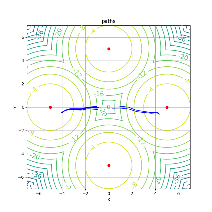
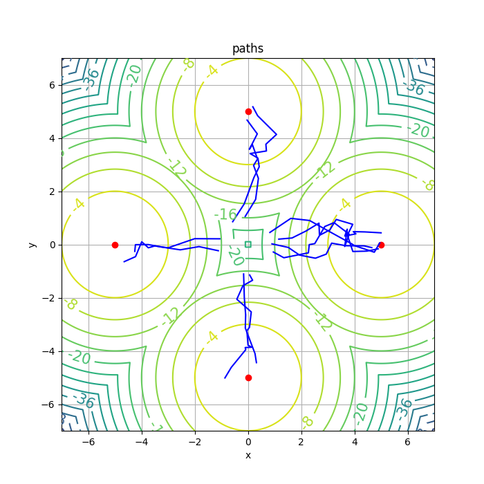
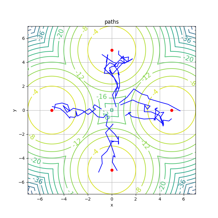
Generally speaking, when \(\alpha\ne 0\), SQL tends to have a high variance, which can also be viewed as the cost for exploration.
4. Conclusion
It was proven that bringing in the entropy term does work for the end of better exploring. The author successfully extended the entropy RL framework to contiunous case in this paper. However, the high variance makes it challenging to be used for performing complicated tasks, and that may be one of the reasons why little (relatively) ink has been spilled on SQL. A wise choice could be to use SQL as an initializer rather than a trainer.
5. References
Reinforcement Learning with Deep Energy-Based Policies - Tuomas Haarnoja et al.
Soft Actor-Critic - Tuomas Haarnoja et al.
Learning Diverse Skills via Maximum Entropy Deep Reinforcement Learning - BAIR
Deep Reinforcement Learning - Julien Vitay
Maximum Entropy Reinforcement Learning (Stochastic Control) - Dongmin Lee
Stein Variational Gradient Descent: A General Purpose Bayesian Inference Algorithm - Qiang Liu and Dilin Wang