This is a brief summary about graphics pipeline based on the first four assignments of the course Games101. The course is educational and friendly to people who is very new to this field like me. Thanks to this, I now finally have a basic understanding of graphics pipeline from a much more practical perspective. This post will cover some concepts about application, geometry, and rasterization of a graphics pipeline (Fig 1) in an (trying to be) intuitive and straightforward way.

Figure 1. Graphics Pipeline (Wikipedia)

1. Application
2. Geometry Processing
- 2.1 MVP Transformation
- 2.2 Viewport Transformation
3. Rasterization
- 3.1 Triangle Traversal
- 3.2 Pixel Shading
4. Conclusion

1. Application

During the application stage, there will be computation such as collision detection, animation, acceleration, and dealing with inputs, etc. The output data should contain the information like positions of vertices, normal information, and colour information an so on.

Example 1.1: In assignment 2, we are required to draw two triangles on the screen, and the data we need is the positions of the six vertices, the indices that determine the components of each triangle, and the colour of each vertices. Here we get the data directly without extra computation.

std::vector<Eigen::Vector3f> pos		// positions of vertices
{
    {2, 0, -2},
    {0, 2, -2},
    {-2, 0, -2},
    {3.5, -1, -5},
    {2.5, 1.5, -5},
    {-1, 0.5, -5}
};

std::vector<Eigen::Vector3i> ind		// vertices' indices of each triangle
{
    {0, 1, 2},
    {3, 4, 5}
};

std::vector<Eigen::Vector3f> cols		// color of each vertices
{
    {217.0, 238.0, 185.0},
    {217.0, 238.0, 185.0},
    {217.0, 238.0, 185.0},
    {185.0, 217.0, 238.0},
    {185.0, 217.0, 238.0},
    {185.0, 217.0, 238.0}
};

rasterizer.load_positions(pos);
rasterizer.load_indices(ind);
rasterizer.load_colors(cols);

2. Geometry Processing

The geometry processing step is responsible for most of the operations with triangles and their vertices. In the assignments, there are mainly two tasks during this stage.

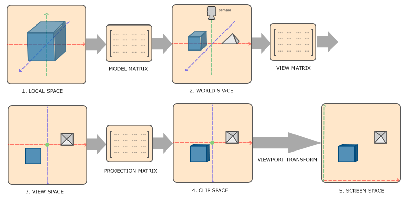
Figure 2. MVP Transformation and Viewport Transformation

2.1 MVP Transformation

Model Transformation: Transforming the vertices of the objects we want to render. Most time this means applying scaling, translation, and rotation. This can be generally done by using three well-defined matrix in the homogeneous coordinates. One can also derive each matrix manually by solving simple equations.

Scale matrix:

\[S(s_x, s_y, s_z)=\begin{bmatrix}s_x & 0 & 0 & 0 \\ 0 & s_y & 0 & 0 \\ 0 & 0 & s_z & 0\\ 0 & 0 & 0 & 1\end{bmatrix};\]

Translation matrix:

\[T(t_x, t_y, t_z)=\begin{bmatrix}1 & 0 & 0 & t_x \\ 0 & 1 & 0 & t_y \\ 0 & 0 & 1 & t_z\\ 0 & 0 & 0 & 1\end{bmatrix};\]

Rotation matrix (rotate counter-clockwise by \(\alpha\) degree):

\[R_x(\alpha)=\begin{bmatrix} 1 & 0 & 0 & 0 \\ 0 & \cos\alpha & -\sin\alpha & 0 \\ 0 & \sin\alpha & \cos\alpha & 0\\ 0 & 0 & 0 & 1\end{bmatrix},\\ R_y(\alpha)=\begin{bmatrix} \cos\alpha & 0 & \sin\alpha & 0 \\ 0 & 1 & 0 & 0 \\ -\sin\alpha & 0 & \cos\alpha & 0\\ 0 & 0 & 0 & 1\end{bmatrix},\\ R_z(\alpha)=\begin{bmatrix} \cos\alpha & -\sin\alpha & 0 & 0 \\ \sin\alpha & \cos\alpha & 0 & 0 \\ 0 & 0 & 1 & 0\\ 0 & 0 & 0 & 1\end{bmatrix}.\]

Example 2.1: In assignment 1, we are required to render a triangle supporting keyboard input. When the key ‘a’ and ‘d’ are pressed, the triangle should be rotated counter-clockwise and clockwise by 10 degrees around \(z\)-axis, respectively. Therefore we have the model transformation matrix as:

Matrix model = Identity();
Update model according to R_z(alpha) defined above;

Viewing Transformation: Transforming all the vertices of the objects in a space where the camera is located at the origin. More specifically, we want the position, gaze direction, and up direction of the camera represents the origin, \(-z\)-axis, \(y\)-axis of the new space, respectively. Obviously, it can be done by applying translation (for the origin) and rotation (for the axes). One can derive the transformation matrix by considering its inverse transformation, especially for its rotation matrix. By doing viewing transformation, we can greatly simplify the computation for projection.

Projection Transformation: Transforming all the vertices of the objects into a normalized device coordinates (NDC) which is \([-1, 1]^3\). By doing so, we can perform projection and clipping more efficiently. For the orthographic projection where all the objects to be projected are in a cuboid space (with top and bottom at \(t\) and \(b\), left and right at \(l\) and \(r\), near and far at \(n\) and \(f\)), the transformation matrix to get NDC is given as

\[M_{NDC}=\begin{bmatrix} \frac{2}{r-l} & 0 & 0 & 0 \\ 0 & \frac{2}{t-b} & 0 & 0 \\ 0 & 0 & \frac{2}{n-f} & 0\\ 0 & 0 & 0 & 1\end{bmatrix} \begin{bmatrix} 1 & 0 & 0 & -\frac{r+l}{2} \\ 0 & 1 & 0 & -\frac{t+b}{2} \\ 0 & 0 & 1 & -\frac{n+f}{2}\\ 0 & 0 & 0 & 1\end{bmatrix}.\]

This matrix can be easily derived manually. Then for orthographic projection, we can just drop the \(Z\) coordinate to get the projection (but with incorrect aspect ratio). For perspective projection where the parallel lines are not parallel in the image space and the projection space is actually a frustum (can be represented by field of view, aspect ratio, near and far planes), we can firstly squish the frustum into a cuboid and then do the orthographic projection. The squish matrix is given as

\[M_{persp->ortho} =\begin{bmatrix} n & 0 & 0 & 0 \\ 0 & n & 0 & 0 \\ 0 & 0 & n + f & -nf \\ 0 & 0 & 1 & 0\end{bmatrix}.\]

Example 2.2: In assignment 1, we are required to render a triangle with perspective projection. The projection matrix is implemented as:

Matrix projection = Identity();

Matrix persp = Identity();
Set persp according to M_{persp->ortho} defined above;

Matrix ortho = Identity();
Set ortho according to M_{NDC} defined above;

projection = ortho * persp;

The resulting \(Z\) coordinate will not be stored in the image, but are only used in depth buffer in the later stages.

2.2 Viewport Transformation

The projection we obtained from MVP transformation after dropping \(Z\) coordinate is in the space \([-1, 1]^2\) with wrong aspect ratio. Viewport transformation helps us to get a correct image on the screen with is \([0, width)\times [0, height)\).

Example 2.3: In almost all the four assignments, the viewport transformation is done by scaling the coordinates:

for each vertex in NDC:
    vertex.x = width * (vertex.x + 1) / 2;
    vertex.y = height * (vertex.y + 1) / 2;
    // z coordinate will be used in the later steps
    vertex.z = vertex.z * (far - near) / 2 + (far + near) / 2;

3. Rasterization

Now it is time for rasterization. This is about writing colour values into the framebuffer for all the pixels. The complexity varies over how we implement texturing, blending, and anti-aliasing, etc. In the assignments, we mainly focus on two tasks (from a very high level): triangle traversal and pixel shading.

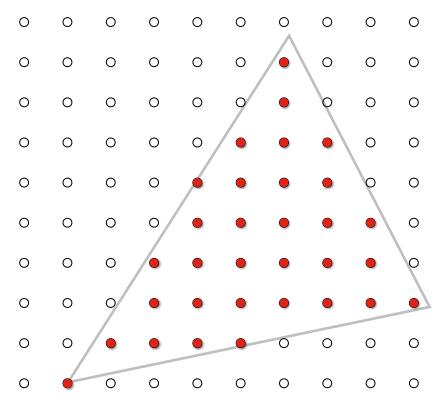
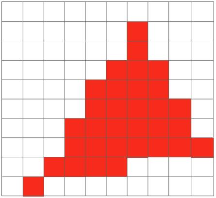
Figure 3. Rasterization

3.1 Triangle Traversal

After viewport transformation, we got a projection of \([0, width)\times [0, height)\) to be rendered on the screen with \(width \times height\) pixels. For each triangle, we need to traverse all the pixels to determine whether they are in the triangle or not. Together with depth information, each pixel then be referred as a point in a single triangle, and will be shaded based on the information of the triangle. We can leverage cross product to determine whether a point is inside a triangle or not:

Example 3.1: In assignment 2, we are required to draw two triangles on the screen. The implementation for inside check can be done as follows:

bool insideTriangle(Point p, Triangle t):
    // points of `t` are `t0`, `t1`, `t2` (counter-clockwise)
    Define vectors p0 = t0 to p, p1 = t1 to p, p2 = t2 to p;
    temp0 = p0.cross(t0 to t1);
    temp1 = p1.cross(t1 to t2);
    temp2 = p2.cross(t2 to t0);
    return temp0 * temp1 * temp2 > 0;

Example 3.2: Still in assignment 2, the triangle traversal and part of the shading is done as:

void rasterize_triangle(Triangle t):
    Construct a bounding box of t to accelerate the computation;
    for each pixel (w, h) in the bounding box:
        if(insideTriangle(Point(w+0.5, h+0.5), t)):
            // Pixel Shading;

3.2 Pixel Shading

Intuitively, pixel shading is responsible for the colour of each pixel. It can be very simple when the colour of each pixel is given by a predefined value. It can be also very tricky when computing those implicit values such as depth that determines the rendering of the overlap part.

After the triangle traversal, we refer each pixel as a point inside a triangle. But very often, we only have the vertices information of a triangle, and we have no information about an arbitrary point inside the triangle. To get the pixel shaded correctly based on what we have, we need the help of interpolation.

Interpolation: The formal definition of interpolation can be found everywhere. Here I just want to explain it in an intuitive way: interpolation is getting new data based on known data on the same space. The key of (linear) interpolation is finding something like weights that describe the contribution of known data to the new data so that the transition from the constructed new data to known data can be smooth. In our case for triangles, we often use Barycentric coordinates to describe the contribution of each vertex to the new data.

Barycentric Coordinates: For every point \((x, y)\) inside a triangle ABC, we can find a corresponding coordinate \((\alpha, \beta, \gamma), \alpha,\beta,\gamma \ge 0\) and \(\alpha+\beta+\gamma=1\).

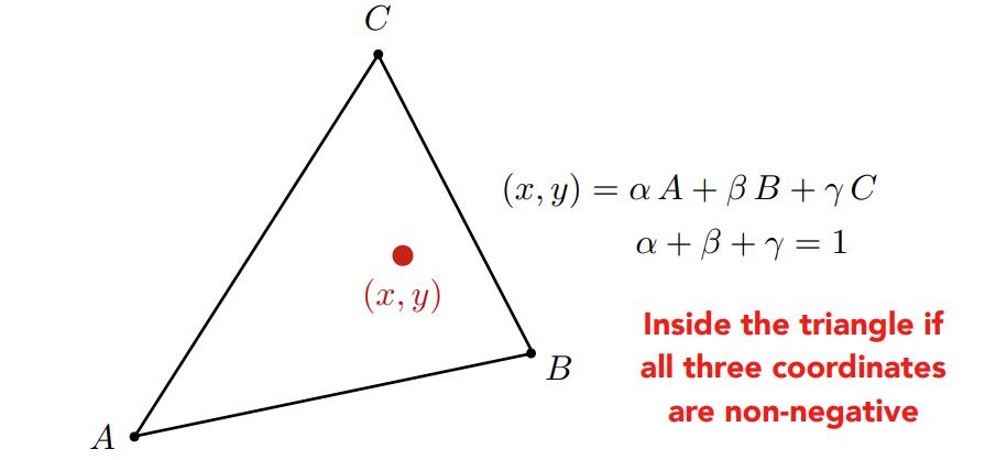
Figure 4. Barycentric Coordinates

The Barycentric coordinates provides us a natural way to capture the weights of the contribution of each vertex of a triangle. Therefore we can interpolate values based on this.

Example 3.3: The triangle traversal in assignment 2 with the interpolation details would be like:

void rasterize_triangle(Triangle t):
    Construct a bounding box of t to accelerate the computation;
    for each pixel (w, h) in the bounding box:
        if(insideTriangle(Point(w+0.5, h+0.5), t)):
            alpha, beta, gamma = compute_Barycentric(Point(w+0.5, h+0.5), t);
            // if the projection is perspective, perspective-correct interpolation should be used
            Get the z value by interpolation;
            if(depth_buffer[w, h] > z):
                // the closer one that should be rasterized
                depth_buffer[w, h] = z;
                frame_buffer[w, h] = color;

As colour of each triangle in assignment 2 is specified, the rendering result on \(700\times 700\) pixels would be like:

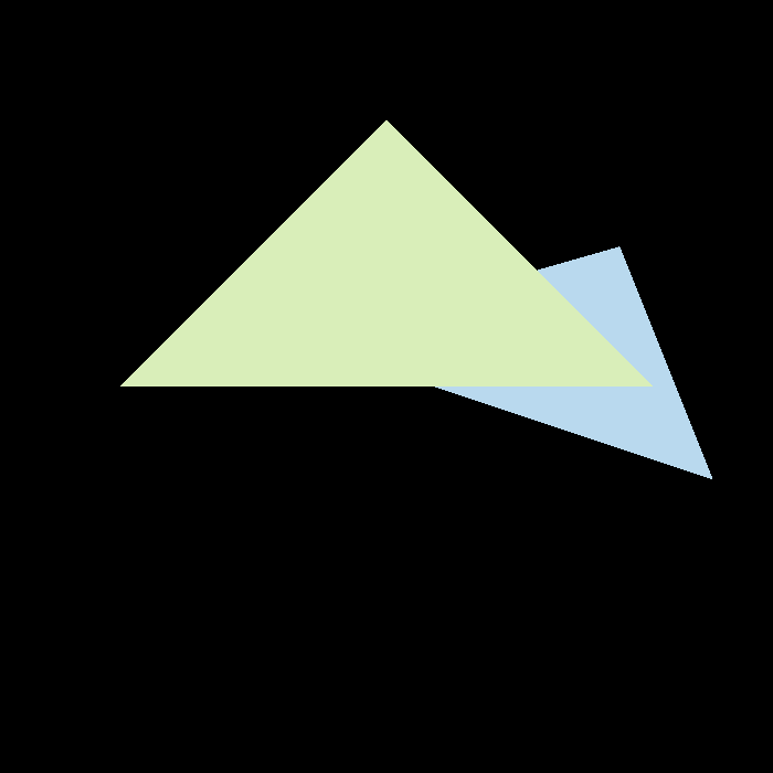
Figure 5. Rasterization of Assignment 2

Notice that there are many jaggies along the edge of the right triangle. That is because each pixel itself is a square and we shade it in a binary way: the colour of it can only be green/blue or black. To remove the jaggies, we should allow each pixel to be shaded in varying colours so that the transition from colourful pixels to black ones can be more smooth. Again, interpolation plays an important role here, but in a different way.

Multi-Sampling Anti-Aliasing (MSAA): In the previous triangle traversal, we traverse each pixel and shade the pixel based on the middle point of the pixel as shown in Fig 6 (a). Therefore for those pixels whose majority part is outside the triangle, the colour will be biased. In MSAA, instead of setting the colour of each pixel based on the middle point, we set it based on \(N\times N\) points inside the pixel. A \(2\times 2\) example is shown in Fig 6 (b). We divide each pixel into four equal parts, and traverse each sub-pixel. The final colour of a pixel will be the average colour of its four sub-pixels.

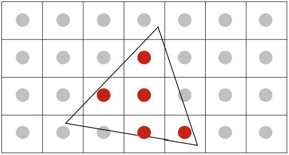
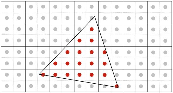
Figure 6. MSAA

Example 3.3: The triangle traversal in assignment 2 with MSAA would be like:

void rasterize_triangle(Triangle t):
    Construct a bounding box of t to accelerate the computation;
    for each pixel (w, h) in the bounding box:
        int count = 0;
        for each sub-pixel (w_, h_) in the pixel (w, h):
            if(insideTriangle(Point(w_+0.25, h_+0.25), t)):
                Get the z value by Barycentric interpolation;
                if(depth_buffer[w_, h_] > z):
                    // the closer one that should be rasterized
                    depth_buffer[w_, h_] = z;
                    count++;
        if(count):
            frame_buffer[w, h] += color * count / 4;

The rendering result with MSAA is shown in Fig 7. In MSAA, we need to maintain a depth buffer for all the sub-pixels. Otherwise there will be black squares along the overlap edge as we shrink the colour values of the pixel by the averaging operation.

Fig 7. MSAA of Assignment 2

All the examples we provide above do not require a specific shading inside a triangle, which means all the pixels of a triangle will be in the same colour. In most cases, the colour of a triangle varies from pixel to pixel. And if we have no information about the vertex colour inside a triangle, we can, again, get one by interpolation. We now discuss four different shaders.

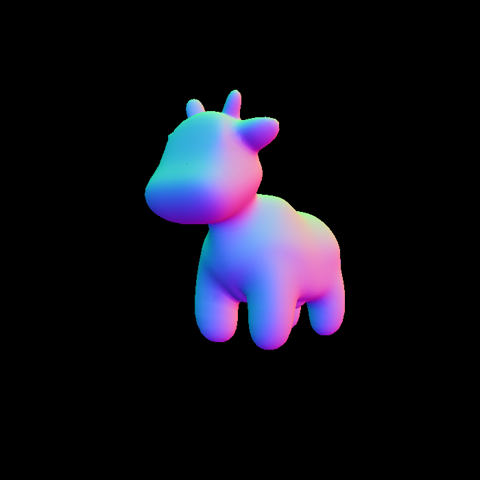
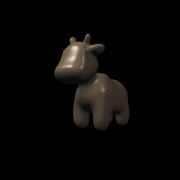
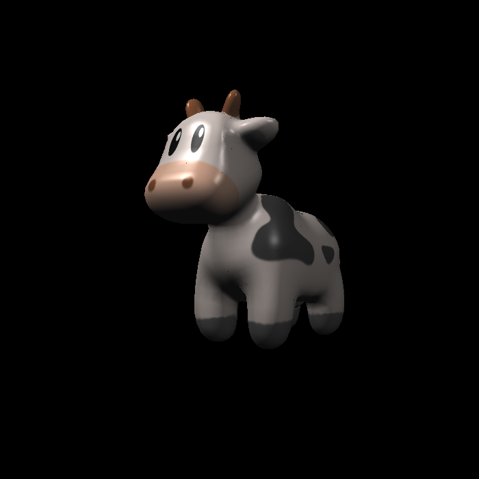
Fig 8. Shaders

Normal Shader: Consider the case where we want to shade each pixel based on the normal of the point to which it is corresponding. All the normal of the inside points are obtained by interpolation.

Example 3.4: In assignment 3, we are provided with a basic normal shader. It works as follows

Vector3f normal_shader(Vector3f normal):
    Vector3f color = 255 * (normal + Vector3f(1.0f, 1.0f, 1.0f)) / 2.0f;
    return color;

void rasterize_triangle(Triangle t):
    Construct a bounding box of `t` to accelerate the computation;
    for each pixel (w, h) in the bounding box:
        if(insideTriangle(Point(w+0.5, h+0.5), t)):
            Get the z value by Barycentric interpolation;
            Get the normal of the point Point(w+0.5, h+0.5) by Barycentric interpolation;
            color = normal_shader(normal);
            if(depth_buffer[w, h] > z):
                // the closer one that should be rasterized
                depth_buffer[w, h] = z;
                frame_buffer[w, h] = color;

The rendering result is shown Fig 8 (a). The blue part indicates the triangles on that part are generally perpendicular to the view ray, and their normal is more like \({0, 0, 1}\), which hence makes them more blue. The normal information can also be obtained from normal map. It is very common to use normal map to trick human eyes that there are a great many surface details. (See bump shader and displacment shader.)

Blinn-Phong Shader: Blinn-Phong shader is based on Blinn-Phong reflectance model. It allows us to take lights into consideration without bringing in too much computation cost. In Blinn-Phong reflectance model, the reflection consists of Lambertian Diffuse, Blinn-Phong Specular, and Ambient. Intuitively, Lambertian diffuse assumes the shading is independent of the view direction, and the ray direction will only affect the intensity of the light. Blinn-Phong specular assumes the view direction will also affect the light intensity at the shading point, and the closer the view direction is to the mirror direction of the ray direction, the higher the intensity at the point. Ambient can be viewed as a constant to simulate the whole environmental reflectance.

Example 3.5: In assignment 3, we are required to implement a Phong shader. To simplify the computation, I implement a Blinn-Phong shader as follows:

Vector3f blinn_phong_shader(Fragment_Shader_Payload payload):
    // pre-define the parameters of ambient, diffuse, and specular as `ka`, `kd`, `ks`
    // assume `normal` is the normal of the shading point
	
    Vector3f color = {0, 0, 0};
	
    // Ambient
    color += ka * ambient_light_intensity;
	
    for each light source:
        Vector3f light_vec = light.position - point;
        Vector3f view_vec = eye.position - point;
        Vector3f bisector = (light_vec + view_vec).normalized();
		
        // Lambertain diffuse
        float r2 = light_vec.dot(light_vec);	// the distance
        color += kd.crossProduct(light.intensity) / r2 * max(0, normal.dot(light_vec.normalized())); 
		
        // Specular
        color += ks.crossProduct(light.intensity) / r2 * max(0, normal.dor(bisector)^150);
		
    return color;

The rendering result is shown Fig 8 (b). As we can see, the image now can show us the reflectance, which makes it more realistic.

Texture Shader: Now consider that we want to have colourful patterns rather than normal or reflectance. One way to specify the colour is by using texture map. Texture shader is usually the same as the Blinn-Phong shader. The only difference is that the parameter \(k_d\) for Lambertian diffuse is replaced by the one extracted from a texture map.

Example 3.6: In assignment 3, we are required to implement a Texture shader. It can be done by modifying Blinn-Phong shader as follows:

Vector3f texture_shader(Fragment_Shader_Payload payload):
    // pre-define the parameters of ambient, diffuse, and specular as `ka`, `kd`, `ks`
    // assume `normal` is the normal of the shading point
	
    kd = payload.texture.getColor(u, v) / 255.f;
	
    Vector3f color = {0, 0, 0};
	
    // compute color based on Blinn-Phong reflectance model
		
    return color;

The rendering result is shown in Fig 8 (c). However, if we zoom in the resulting image, we can tell that there are jaggies again in the result. Instead of using MSAA, we can use Bilinear interpolation here to remove jaggies. The idea of Bilinear interpolation is shown in Fig 9. It is trying to get an averaging colour so that the transition from one pixel to the other can be as smooth as possible. The rendering result of Bilinear interpolation is shown in Fig 8 (d).

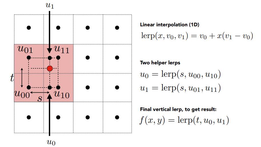
Figure 9. Bilinear Interpolation

4. Conclusion

This post is a hasty summary about graphics pipeline after my completing the first four assignments. Before this, though I had read many articles about graphics pipeline, some concepts were very abstract to me. After getting hands dirty, I finally have a practical perspective about how we draw things literally. Many thanks to this great course!