Machine Learning - 08 Probabilistic Graphical Models
The notes are based on the session and PRML. For the fundamental of probability, one can refer to Introduction to Probability. Many thanks to these great works.
0. Introduction
For a vector featured with multiple random variables like \(X=[x_1,x_2,\dots,x_n]\), what we care most are marginal probability \(P(x_i)\), joint distribution \(P(X)\) and conditional probability \(P(x_i\vert x_j)\):
-
Marginal distribution:
\[P(x_i)=\sum_{x_n}\dots\sum_{x_{i+1}}\sum_{x_{i-1}}\dots\sum_{x_1}P(X);\] -
Joint distribution:
\[P(X)=P(x_1)\cdot\prod_{i=2}^{n}P(x_i\vert x_1,\dots,x_{i-1});\] -
Conditional probability (Bayesian rule):
\[P(x_i\vert x_j)=\frac{P(x_i,x_j)}{P(x_j)}.\]
Obviously when \(n\) is large, all of the above three can be of high computation complexity. Now we consider simplifying the computation of joint distribution, and to achieve that most methods have been proposed by
-
assuming all the features are totally independent:
\[P(X)=\prod_{i=1}^nP(x_i);\] -
or, assuming that the features are conditional independent, which is used in naive Bayes classifier as class conditional independence:
\[P(X\vert Y)=\prod_{i=1}^n P(x_i\vert Y)\implies P(X)=\int_y \prod_{i=1}^nP(x_i\vert y)P(y)\text{d}y;\] -
or, based on conditional independent, assuming that the features process the Markov Property, which is used in hidden Markov models:
\[P(x_j\vert x_1,x_2,\dots,x_{j-1})=P(x_j\vert x_{j-1})\implies P(X)=P(x_1)\cdot\prod_{i=2}^nP(x_i\vert x_{i-1}).\]
Among them, graphical probabilistic models (PGM) are generally based on the conditional independence assumption, ‘capturing the way in which the joint distribution over all of the random variables can be decomposed into a product of factors each depending only on a subset of the variables’. (PRML)
By leveraging the manipulations and properties of graph, many probabilistic insights can be obtained, motivating the design of new models.
1. Bayesian Networks
We now consider general graphical probabilistic models Bayesian networks which are defined by directed acyclic graphs (DAGs). Given a DAG, the nodes in a Bayesian network represent random variables and edges represent conditional dependencies among those variables.
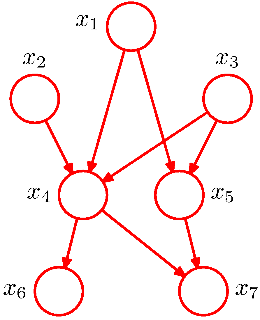
Figure 1. Example of a directed acyclic graph (Figure 8.2 of PRML).
A Bayesian network actually represents a joint distribution over all the random variables represented by its nodes. As it is shown in Figure 1 (from PRML), there are 7 random variables. The edge going from a node \(x_i\) to a node \(x_j\) indicates that \(x_j\) is dependent to \(x_i\). The joint distribution of the model in Figure 1 is then given by
\[P(x_1,x_2,\dots,x_7)=P(x_1)P(x_2)P(x_3)P(x_4\vert x_1,x_2,x_3)P(x_5\vert x_1,x_3)P(x_6\vert x_4)P(x_7\vert x_4,x_5).\]More generally, for a graph with \(K\) nodes, the corresponding joint distribution is given by
\[P(X)=\prod_{k=1}^KP(x_k\vert \mathbb{Pa}_k),\]where \(\mathbb{Pa}_k\) denotes the set of parents of \(x_k\) and \(X=(x_1,x_2,\dots,x_k)\). Such a key equation expresses the factorization properties of the joint distribution for a directed graph. Compared with the joint distribution expression mentioned in Section 0, the expression of that of Figure 1 we show above definitely is simplified a lot. Such simplification is actually introduced by the absence of edges in the graph, which conveys the conditional independence information of those variables.
1.1. Conditional Independence
Conditional independence sometimes can greatly simplify the computations needed to perform inference and learning under probabilistic models. By using graphical models, we can find the conditional independence properties directly without effort to any analytical manipulations. We start the discussion by considering three simple examples each involving graphs having just three nodes.
1.1.1. Tail-to-tail
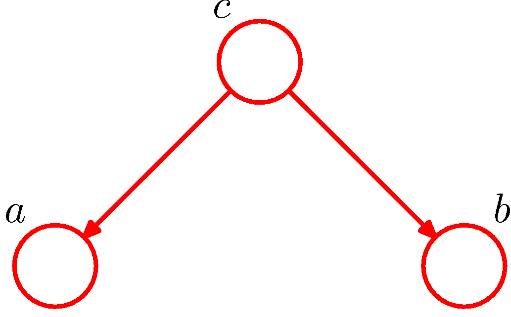
Figure 2. Example of tail-to-tail for conditional independence (Figure 8.15 of PRML).
Intuitively, we can consider the path from node a to node b via c in Figure 2. The node c is said to be tail-to-tail as the node is connected to the tails of the two arrows. Given such a path, we have \(a\) and \(b\) dependent. However, if we condition on node c, then the conditioned node c will block the path and cause \(a\) and \(b\) to become conditionally independent. A naive proof is as follows.
By the definition given in section 1, the joint distribution of the graph in Figure 2 is
\[P(a,b,c)=P(c)P(a\vert c)P(b\vert c).\]By the general definition of the marginal distribution, we have
\[P(a,b)=\sum_c P(c)P(a\vert c)P(b\vert c),\]which generally dose not factorize into the product \(P(a)\cdot P(b)\), therefore \(a\) and \(b\) are dependent, denoted as
\[a\not\perp b\ \ \ \ \ \ \text{or, equivalenly,}\ \ \ \ \ \ a\not\!\perp\!\!\!\perp b\vert \emptyset.\]By the general definition of the joint distribution, we have
\[P(a,b,c)=P(c)P(a\vert c)P(b\vert a,c).\]Thus it follows that
\[\begin{alignat*}{3}&&P(c)P(a\vert c)P(b\vert a,c)&=P(c)P(a\vert c)P(b\vert c)\\\implies&&P(b\vert a,c)&=P(b\vert c)\\\implies&&\frac{P(a,b\vert c)}{P(a\vert c)}&=P(b\vert c)\\\implies&&P(a,b\vert c)&=P(a\vert c)P(b\vert c),\end{alignat*}\]which means
\[a\perp\!\!\!\perp b\vert c.\]1.1.2. Head-to-tail

Figure 3. Example of head-to-tail for conditional independence (Figure 8.17 of PRML).
The example of head-to-tail is shown in Figure 3. Similarly, the node c is said to be head-to-tail with respect to the path from node a to node b. Given such a path, we have \(a\) and \(b\) dependent. When node c is conditioned, the case would be the same as tail-to-tail: the conditioned node c would block the path and render \(a\) and \(b\) conditional independent. The naive proof of this is as follows.
The joint distribution of the model in Figure 3 is
\[P(a,b,c)=P(a)P(c\vert a)P(b\vert c).\]Marginalizing the distribution over \(c\), we have
\[\begin{aligned}P(a,b)&=\sum_c P(a)P(c\vert a)P(b\vert c)\\&=P(a)\sum_c P(b,c\vert a)\\&=P(a)P(b\vert a),\end{aligned}\]which means \(a\not\perp b\).
By rewriting the general joint distribution expression, we have
\[P(a,b,c)=P(a)P(b\vert a)P(c\vert a,b).\]Then we have
\[\begin{alignat*}{3}&&P(a)P(b\vert a)P(c\vert a,b)&=P(a)P(c\vert a)P(b\vert c)\\\implies&& P(b\vert a)\cdot\frac{P(a,b\vert c)P(c)}{P(b\vert a)P(a)}&=\frac{P(a\vert c)P(c)}{P(a)}\cdot P(b\vert c)\\\implies&&P(a,b\vert c)&=P(a\vert c)P(b\vert c)\\\implies&&a&\perp\!\!\!\perp b\vert c.\end{alignat*}\]1.1.3. Head-to-head
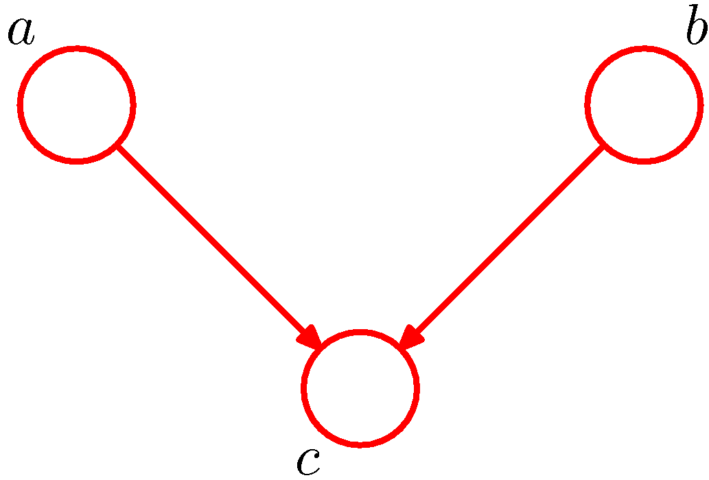
Figure 4. Example of head-to-head for conditional independence (Figure 8.19 of PRML).
The third example given in Figure 4 is opposite to the previous two cases. The node c in Figure 4 is head-to-head with respect to the path from a to b as it connects to the heads of the two arrows. In this case, node c would block the path while conditioning on node c would unblock the path and render \(a\) and \(b\) dependent. The proof is much similar to the previous cases.
The joint distribution of the model in Figure 4 is
\[P(a,b,c)=P(a)P(b)P(c\vert a,b).\]Marginalizing the distribution over \(c\), we have
\[\begin{aligned}P(a,b)&=\sum_c P(a)P(b)P(c\vert a,b)\\&=P(a)P(b)\sum_c P(c\vert a)\\&=P(a)P(b)\end{aligned}\]which means \(a\perp b\). In particular, the third equation is given by the fact ‘conditional probabilities are probabilities’ (Introduction to Probability).
By rewriting the general joint distribution expression, we have
\[P(a,b,c)=P(a,b\vert c)P(c).\]Then we have
\[\begin{alignat*}{3}&&P(a,b\vert c)P(c)&=P(a)P(b)P(c\vert a,b)\\\implies&&P(a,b\vert c)&=\frac{P(a)P(b)P(c\vert a,b)}{P(c)},\end{alignat*}\]where the last term in general does not factorize into the product \(P(a\vert c)P(b\vert c)\), hence we have
\[a\not\!\perp\!\!\!\perp b\vert c.\]1.1.4. D-separation
With the three examples, we now introduce D-separation which is used to determine the independence of those random variables in a graph. Specifically, given three arbitrary nonintersecting sets \(\mathcal{A}\), \(\mathcal{B}\) and \(\mathcal{C}\) of the nodes of the graph, by D-separation we can determine whether the statement \(\mathcal{A}\perp\!\!\!\perp\mathcal{B}\vert \mathcal{C}\) is true under the graph.
The method proceeds as follows. (I am sure this great video can help you get into D-separation easily.)
- Find out all possible undirected paths between any node in \(\mathcal{A}\) and any node in \(\mathcal{B}\);
- Check whether those paths are blocked: for each path,
- splitting it into continuous triples;
- for each triple, its structure (with directionality concerns) must belong to one of the three examples we mentioned before, and we just need to determine whether it is blocked when conditioning on \(\mathcal{C}\);
- if there is at least one triple blocked, the path is said to be blocked, otherwise, the path is unblocked;
- If all the paths are blocked, the statement \(\mathcal{A}\perp\!\!\!\perp\mathcal{B}\vert \mathcal{C}\) is true and \(\mathcal{A}\) is said to be d-separated from \(\mathcal{B}\) by \(\mathcal{C}\).
1.2. Markov Blanket
We now introduce the concept of a Markov blanket or Markov boundary. Consider a joint distribution \(P(x_1,x_2,\dots,x_N)\) represented by a directed graph having \(N\) nodes. In particular, we want to determine the conditional distribution
\[P(x_i\vert x_{\{j\ne i\}})=\frac{\prod_k P(x_k\vert \mathbb{Pa}_k)}{\int\prod_k P(x_k\vert \mathbb{Pa}_k)\text{d}x_i}.\]Notice that if the term \(p(x_k\vert \mathbb{Pa}_k)\) does not involve \(x_i\), that is to say \(k\ne i\) and/or \(x_i\notin\mathbb{Pa}_k\), we then can remove the term from both numerator and denominator. The remaining terms in the conditional distribution then must be
\[P(x_k\vert \mathbb{Pa}_k), k\in\{i\}\cup\{k\vert x_i\in\mathbb{Pa}_k\},\]and the conditional distribution \(P(x_i\vert x_{\{j\ne i\}})\) depends only on those terms. We now discuss which nodes those terms are related to. Obviously, when \(k\in\{i\}\), the term \(P(x_i\vert \mathbb{Pa}_i)\) would only involve \(x_i\) and the parents of it. When \(k\in\{j\vert x_i\in\mathbb{Pa}_j\}\) and \(k\ne i\), the term \(P(x_k\vert \mathbb{Pa}_k)\) are related to two parts. The first part \(x_k\) is the child of \(x_i\) as \(x_i\in\mathbb{Pa}_k\), while the second part \(\mathbb{Pa}_k\) is the co-parents of the child \(x_k\).
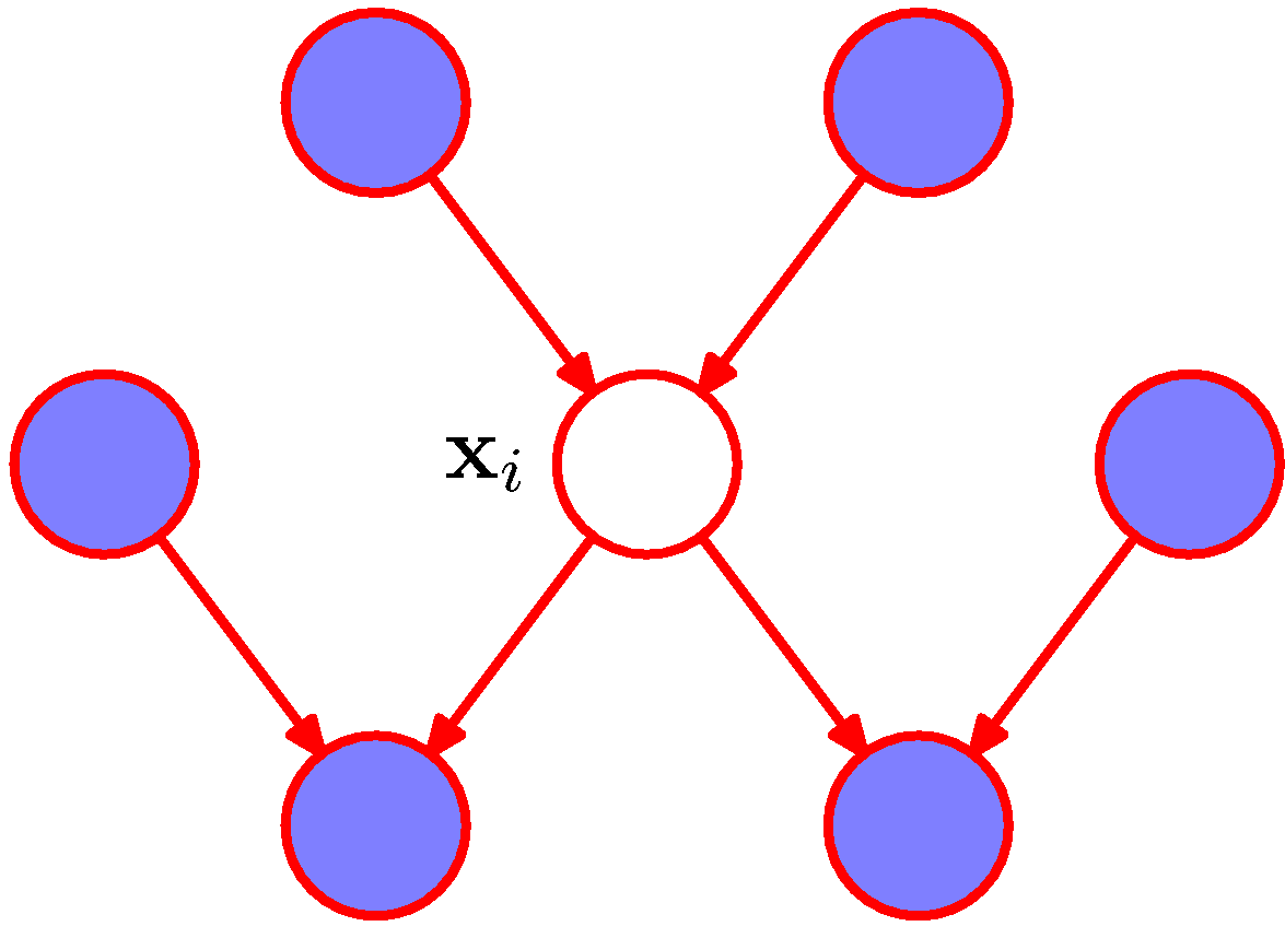
Figure 5. The Markov blanket of $$x_i$$ is denoted by colored nodes. (Figure 8.26 of PRML).
As shown in Figure 5, we say that a Markov blanket \(\mathcal{M}_i\) of a node \(x_i\) comprises the set of its parents, child and co-parents. Given the Markov blanket, the conditional distribution \(P(x_i\vert x_{\{j\ne i\}})\) can be rewritten as \(P(x_i\vert \mathcal{M}_i)\).
2. Markov Network
The graphs we talked in the previous sections are directed. When it comes to undirected graphs, some concepts of directed graphs still play important roles while others do not. The graphical probabilistic models defined by undirected graphs is called Markov networks, also known as Markov random fields. Similar to Bayesian networks, the nodes in a Markov network represent random variables. However, as edges carry no arrows in undirected graphs, the function of edges changes a lot.
2.1. Conditional Independence
The conditional independence of an undirected graph is given by the absence of edges. Specifically, for a graph with nodes representing random variable \(x_1,x_2,\dots, x_N\), we have:
Pairwise Markov Property: the absence of an edge between two nodes \(x_i\) and \(x_j\) means the corresponding random variables of the two nodes are conditionally independent given all the other random variables, which is
\[x_i\text{ and }x_j\text{ are not adjacent}\implies x_i\perp\!\!\!\perp x_j\vert X_{\setminus \{i,j\}},\]where \(X_{\setminus\{i,j\}}\) denotes the set of all the variables with \(x_i\) and \(x_j\) removed.
Local Markov Property: a random variable \(x_i\) is conditionally independent of all other random variables given its neighbors, which is
\[x_i\perp\!\!\!\perp X_{\setminus \mathbb{Ne}_i}\vert \mathbb{Ne}_{i},\]where \(\mathbb{Ne}_i\) is the set of neighbors of \(x_i\), i.e., every node directly connected with \(x_i\) is in \(\mathbb{Ne}_i\). Recalling the definition of the Markov blanket, we can find that \(\mathbb{Ne}_i\) is the Markov blanket in the undirected graph.
The property below is to Markov networks as D-separation is to Bayesian networks
Global Markov Property: for any three nonintersecting sets \(\mathcal{A}\), \(\mathcal{B}\) and \(\mathcal{C}\) of the nodes of the graph, we can determine whether
\[\mathcal{A}\perp\!\!\!\perp \mathcal{B}\vert\mathcal{C}\]by the following steps:
- Find out all possible paths between any node in \(\mathcal{A}\) and any node in \(\mathcal{B}\);
- Check whether every path from \(\mathcal{A}\) to \(\mathcal{B}\) passes through at least one node in \(\mathcal{C}\);
- If so, the statement is true.
Notice that compared with Bayesian networks, the way we check a statement of the conditional independence in Markov networks actually does not entail the concept ‘block’. Testing for conditional independence in undirected graphs is therefore simpler than in directed graphs.
It can be shown that the three properties above are equivalent.
2.2. Maximum Clique
As a Bayesian network can represent a joint distribution over finite random variables, there also exists a probability density function for each Markov network that is consistent with the three properties we mentioned above. Before moving on, we introduce a concept for a Markov network called a clique, which is defined as a subset of fully connected notes of the undirected graph. Obviously, there may be many different cliques for a Markov network. Among them, we particularly focus on the cliques each of which allows no other nodes to be added without it ceasing to be a clique, and we call such a clique a maximal clique.
Denote the maximal cliques set of a Markov network with \(\{x_1,x_2,\dots,x_N\}\) by \(C_m=\{C\vert C\text{ is a maximal clique}\}\), and the nodes in maximal clique \(C\) by \(\text{x}_C=\{x_i\vert x_i\in C\}\). Then the joint distribution represented by the Markov network can be written as
\[P(x_1,x_2,\dots,x_N)=\frac{1}{Z}\prod_{C}^{C_m}\psi_C(\text{x}_C),\]where \(\psi_C(\cdot)\) are positive functions called potential functions, and the quantity \(Z\) is called partition function that validates the distribution, i.e.,
\[Z=\sum_x\prod_C^{C_m}\psi_C(\text{x}_C).\]Given a Markov network, the equivalence of the joint distribution and the conditional independence can be shown by Hammesley-Clifford theorem.
We now consider the choice of potential functions. Given the existence of partition function, we have great flexibilities in choosing potential functions. However, it naturally raises the question of how to motivate a choice of potential function for a particular application. Since it requires the potential functions to be positive, a widely used function is exponential function:
\[\psi_C(\text{x}_C)=\exp\{-E(\text{x}_C)\},\]where \(E(\text{x}_C)\) is called energy function. The joint distribution then is
\[\begin{aligned}P(x_1,x_2,\dots,x_N)&=\frac{1}{Z}\prod_{C}^{C_m}\psi_C(\text{x}_C)\\&=\frac{1}{Z}\exp\left\{-\sum_{C}^{C_m}E(\text{x}_C)\right\},\end{aligned}\]which is known as Boltzmann distribution (or, Gibbs distribution). Moreover, we can see that the distribution is consistent with the definition of exponential families. The joint distribution of any Markov network in which every potential has the form of exponentials is in exponential families.
2.3. Moralization
We now consider the relation between the two graphical models. Particularly, we consider a problem of how to converting a Bayesian network to a Markov network. We start the discussion from the three examples of Bayesian networks mentioned in section 1.
-
Tail-to-tail: Given the tail-to-tail case shown in Figure 2, we have the joint distribution
\[P(a,b,c)=P(c)P(a\vert c)P(b\vert c).\]A factorization can be easily obtained by identifying
\[\begin{aligned}P(a,b,c)&=\psi(a,c)\psi(b,c),\\\psi(a,c)&=P(c)P(a\vert c),\\\psi(b,c)&=P(b\vert c),\end{aligned}\]which is actually the joint distribution represented by the Markov network whose maximum cliques are \(\{a,c\}\) and \(\{b,c\}\) and potential functions are \(\psi(a,c)\) and \(\psi(b,c)\). Obviously, such a Markov network is the same as the Bayesian network in Figure 2 with removing its arrows.
-
Head-to-tail: For the graph in Figure 3, we have
\[P(a,b,c)=P(a)P(c\vert a)P(b\vert c).\]Similarly, by identifying
\[\begin{aligned}\psi(a,c)&=P(a)P(c\vert a),\\\psi(b,c)&=P(b\vert c).\end{aligned}\]We have the corresponding Markov network with maximum cliques \(\{a,c\}\) and \(\{b,c\}\), which also can be obtained by removing the arrows of the graph.
-
Head-to-head: The case shown in Figure 4 is a little tricky. Given the joint distribution
\[P(a,b,c)=P(a)P(b)P(c\vert a,b),\]we can find that the term \(P(c\vert a,b)\) leads to a factor that depends on three nodes. Therefore the corresponding Markov network must have a maximum clique consists of \(\{a,b,c\}\). To this end, we need to not only remove the arrows of the graph but also add an edge between \(a\) and \(b\). Then we have the corresponding Markov network with potential function
\[\psi(a,b,c)=P(a)P(b)P(c\vert a,b).\]
Given the above discussion, to convert a directed graph into an undirected graph, the general steps are
- Remove all the arrows in the directed graph;
- Add additional edges between all pairs of parents for each node;
- Initialize all the potential functions to 1;
- Multiply each conditional distribution factor into the potential function whose corresponding clique contains all the variables of the factor.
The step adding additional edges is known as moralization. And the resulting undirected graph after removing arrows is called moral graph.
3. Factor Graph
Notice that in moralization, we may invite loops in the moral graph, which can be tricky in some cases. To avoid the issues incurred by the loops, we can leverage factor graphs. Given a joint distribution of a moral graph, we can construct a factor graph by
- Remove all the edges in the graph;
- Rewrite the joint distribution as a multiplication of multiple functions where the functions can depend on an arbitrary set of the nodes;
- Add new nodes for each function of the new expression;
- Add edges between each function and the nodes it depends on.
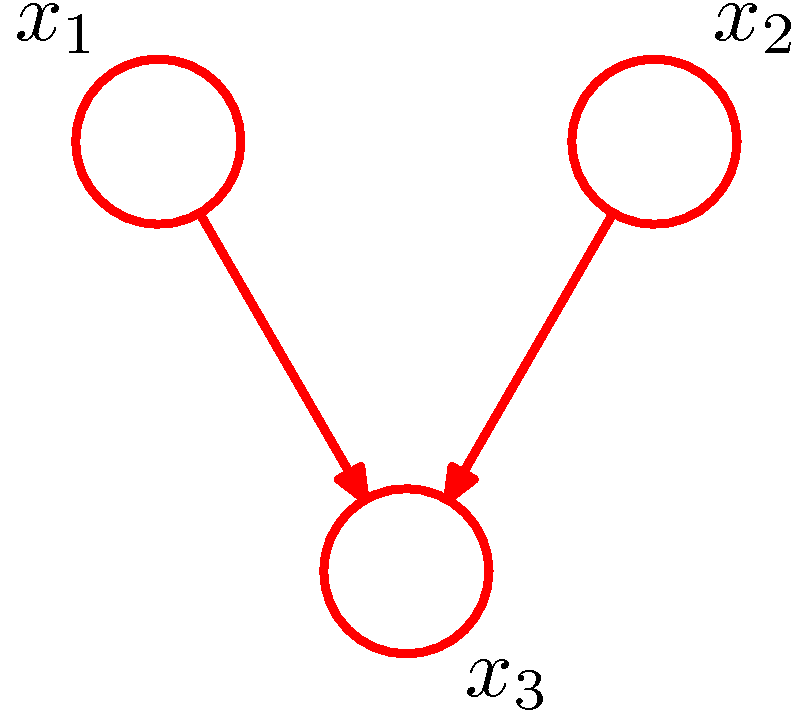
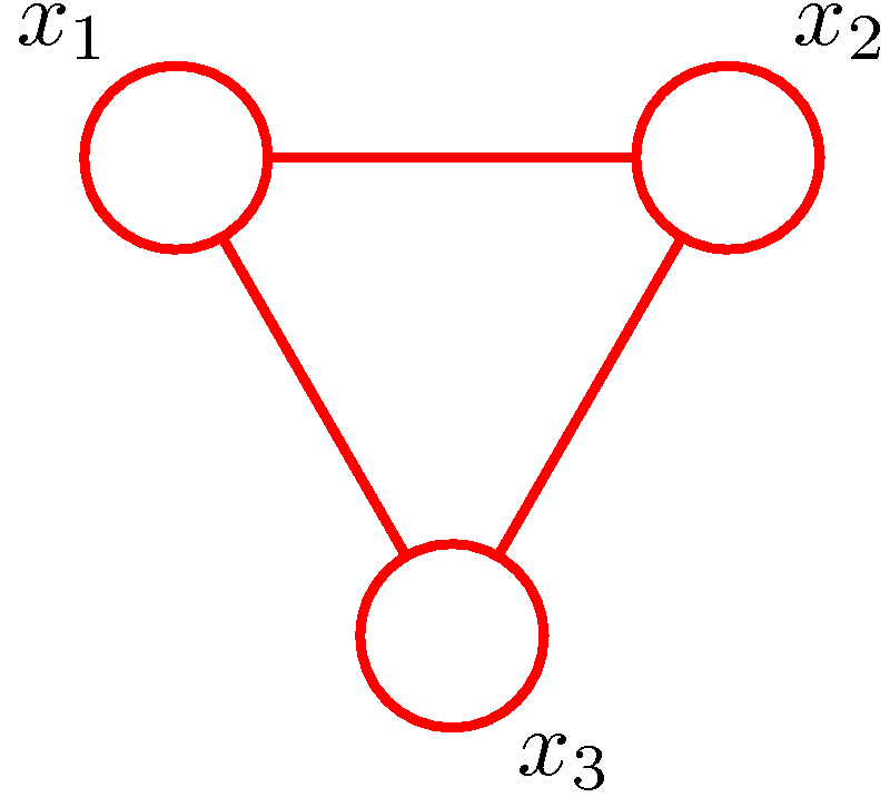
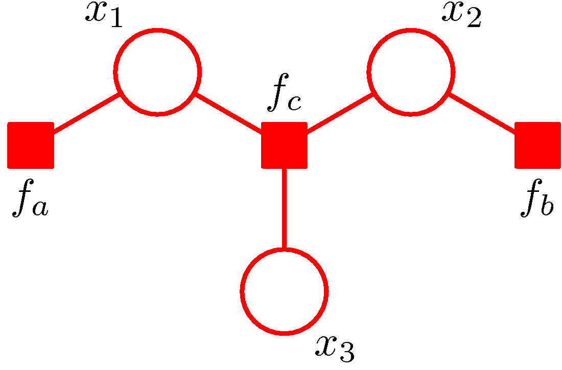
Figure 6. (a) A directed graph. (b) The corresponding moral graph of the directed graph. (c) A factor graph of the graph where the factors are depicted by small solid squares. (Figure 8.41 and Figure 8.42 of PRML).
An example is shown in Figure 6. The directed graph represents the joint distribution
\[P(x_1,x_2,x_3)=P(x_1)P(x_2)P(x_3\vert x_1,x_2).\]The moralization of the directed graph incurs a loop among \(x_1,x_2,x_3\) as shown in Figure 6 (b). Defining \(f_a(x_1)=P(x_1)\), \(f_b(x_2)=P(x_2)\) and \(f_c(x_1,x_2,x_3)=P(x_3\vert x_1,x_2)\), we have
\[P(x_1,x_2,x_3)=f_a(x_1)f_b(x_2)f_c(x_1,x_2,x_3).\]The factor graph corresponding to such a factorization is shown in Figure 6 (c). Moreover, all factor graphs are bipartite as they consist of two distinct kinds of nodes. With factor graphs, we can conduct the related computation based on the factor nodes rather than variable nodes so that the loop can be avoided.
4. Conclusion
In this post, we first introduced two kinds of probabilistic graphical models. One is Bayesian networks that is based on directed acyclic graph. The other is Markov network that is based on undirected graph. Both two models can be used to represent the joint distribution and reflect the conditional independences over a set of random variables. Then we discussed how to convert a Bayesian network into a Markov network. The loops in the moral graph incurred by the conversion can be avoided by transforming the graph into a factor graph.